Geoscientist Online

Kristín Vala Ragnarsdóttir and Harald U Sverdrup* put natural resources into Global Perspective.

In 1971, at the request of the Club of Rome, an MIT systems engineering professor called Jay Forrester developed a model for the future economy, showing that a resource crisis could be imminent.  Aurelio Peccei, an Italian economist and industrialist and former boss of FIAT and Olivetti, realised that a more comprehensive study was needed to address the interplay between three factors - exponential population growth, global resources and environmental pollution. 

Figure 1.  Colin Campbell demonstrates peak oil at an Irish pub.  The full glass represents oil resources in 1900, the half empty glass represents the year 2000, and the near-empty glass oil resources in 2100.   

The Club of Rome, of which Peccei was a founder and president, initiated the work that led to Limits to Growth (1972).  This study was led by Forester´s PhD student Dennis Meadows, with help from Donella Meadows (a biochemist), Jørgen Randers (a physicist) and Willhelm Berents III (an agronomist).  It had a global impact, and sold over 30 million copies in 30 languages. 

But the debate soon became derailed, because LTG suggested curbing economic growth – an unwelcome idea to those who have a large stake in the status quo¹.  Governments fear dwindling tax revenue, while mainstream economists resist any change to the paradigm of eternal growth.  As any businessman knows, managing growth is a lot easier than either of the alternatives.  Meanwhile, neither public nor policymakers appear to grasp that resources form the basis for economic growth. 

ASPO

Oil-company geophysicists Colin Campbell and Jean Laherrere, together with physicist Professor Kjell Aleklett, founded the Association for the Study of Peak Oil (ASPO) in 2001.  Their work built on that of Marion King Hubbert, who in the 1950s developed a model for oil production and field exhaustion, which has since been referred to as ‘peak oil’. Hubbert (correctly!) predicted a peak production date for the oil and energy reserves of the United States as 1970.  Campbell and co tirelessly presented data at conferences showing that we were about to reach peak oil - and indeed this peak was reached in 2006 ^2,3. 

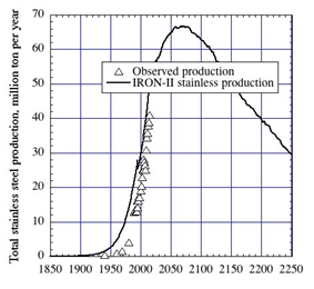
Figure 2.  Data for mining rates and the total mining rate outputs for iron (a, left), nickel (b, right) and stainless steel (c, below), using the WORLD model and the Hubbert’s model (b).  Note that after 2080 recycling will be the dominant source of iron, and that after 2035, recycling is the dominant source of nickel. 

The ecologist Charles Hall has extended the debate by defining the concept of Energy Return on Investment (EROI) for oil, demonstrating that as oil dwindles, so does EROI.  It began with a ratio of over 100 in the 19^th Century, but is going down because it costs more and more energy to get oil out of the ground as reservoirs get deeper (under the sea or ground) and refining costs rise as oil grade declines.  EROI for oil stood around 40 in the US in 2005, is below 10 for deep oil, and around 2 for shale oil.

Meadows et al.  (and updates of their work^4,5,6,7,8) indicated what changes were needed to curb the exponential exploitation of natural resources.  Based on integrated systems analysis and dynamics they presented several scenarios with future options, from which societies and policy makers could choose.  Unfortunately the international community continued with the ‘business as usual’ scenario, generally referred to as ‘the standard run’.  The message of their work was, however, that we must change course before causing irreversible damage to the environment and its life-support systems for billions of people. 

Australian geologist Graham Turner, revisiting the ‘limits to growth’ scenarios ^{9, 10} has demonstrated that we have however continued with the ‘standard run’.  We have recently published a comprehensive analysis, in the October 2014 issue of Geochemical Perspectives¹¹ which asks - do we still have time, or is it too late for a change of direction to do any good?

Methods

We have used several different methods to assess resource availability.  These are, in order of increasing complexity: Burn-off time (business as usual), peak discovery early warning, Hubbert´s model estimates, and systems dynamics modelling.  We describe these briefly  here and at greater length elsewhere ^11,12,13. 

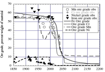
Figure 3.  Production rate for Mn-Cr-Ni-based stainless steel and Mn-Cr steel without nickel (a, left) from the WORLD model.  When we run out of sufficient nickel, stainless steel will be substituted with a simpler quality without it.  (b, right) Data for ore grades (symbols) compared to the outputs from the WORLD model (lines) for iron, manganese, chromium and nickel.  Sverdrup and Ragnarsdottir (2014).

In our work the US Geological Survey is an important source of data and definitions (see below), which we follow.  A list can be found at the end of this online article. 

In our models we work with all technically extractable ore content (below referred to as ‘reserves’) classified according to ore grade and extraction costs.  The result is that that we will experience ever-rising costs as ore quality and extraction yields go down. 

Burn-off time is a ‘worst-case scenario’, and gives an order of magnitude indication for how long the reserves will last.  Burn-off time is defined as estimated extractable reserves divided by the present net yearly extraction rate - the ratio between reserves estimated to be extractable, and present consumption, expressed in years.  It is an indicator, rather than a robust time estimate, and should be used as such. 

Peak discovery early warning: earlier work has shown that there is a systematic shift of 40 years between peak discovery and production peak for a large number of different metals, materials and fossil fuels^12,14.  Thus, when we know the peak year in reserve discovery, we also know, 40 years ahead of time, when the peak production will come  - with a good measure of certainty. 

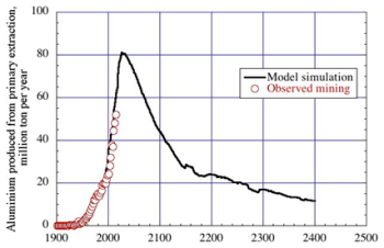
Figure 4.  WORLD model simulation of primary aluminium production rate 1900-2500 using the same extractable amount; Hubbert’s model (a, above left) and the WORLD model (b, right).  Aluminium mining compared to recycling and supply (c, below).  Note the model predicts recycling as the main source of Al after 2020.  Because of relatively efficient recycling, supply is much larger than the mining rate.  WORLD model tested on how well it predicts market price for Al (d, below). 

H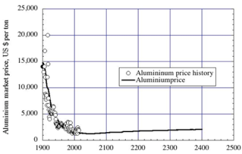ubbert’s model estimates of peak production and time to scarcity was set forth by M  King Hubbert (Shell Oil), when he developed the Hubbert curve, from 1956 on, to predict the lifetime of wells and fields.  He showed, using observed production data for oil wells (as well as uranium and phosphate mining), that all finite metal, material and fossil fuel exploitation follows the distinctive pattern of the Hubbert normal curve.  Hubbert verified this model using field data several times over. 

We have often been told that Hubbert curves ‘cannot be applied to metals’.  But we have tried them on reserves data for more than 40 metals, minerals and materials, and tests on field data demonstrate that they work excellently, on any non-renewable mined geological reserve ¹⁵. 

System dynamic modelling was used to reconstruct the past for explanatory and testing purposes - to estimate time to production maximum, and to study the rate of decline to scarcity, after maximum production has passed.  The flow pathways and the causal chains and feedback loops in the system are mapped using systems analysis, and the resulting coupled differential equations describing these feedbacks are transferred to computer code for numerical solution, using an environment such as STELLA^®.  The methods are those used in systems analysis and systems dynamics for modelling complex systems^{8, 16} .  This method gives more detail, demands more insight and can include more factors, but is more difficult to parameterise. 

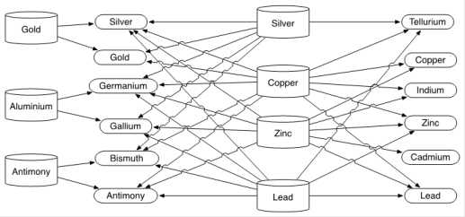
Figure 5.  Interconnected flowchart of the parent ores of copper, zinc and lead, as modelled with BRONZE (submodule of WORLD).  Cylinders represent reserves, ovals the production for each metal.   

The WORLD model, used to produce the runs presented in this study, is similar to the approach taken by Meadows et al. in their World3 model, and presented in LTG.  However, World3 lumped extractable amounts for energy, metals and all materials, missing the dynamics that arise when they are presented as coupled but separate, as here.  Contrary to many claims, the Meadows team did not ‘confuse resources and reserves’ (as defined by the USGS – see online).  Interested readers are pointed to the scientific background document⁴ and Limits to Growth⁵, aimed at the public.  The ‘standard run’ of LTG has been shown, 40 years later, to be correct^9,10.  Materials however can be recycled, whereas much energy cannot.  This is being corrected in our WORLD model, currently under development¹¹.

Metals modelled

Applying our analysis to over 40 natural resources of metals and materials, we find that most have either reached peak production, or will do so before 2050 (See Table 1, available Online).  We have selected to show here the results for some of the metals most important to society: iron (1450 million tons per year primary extraction), manganese (18 million tons per year), chromium (16 million tons per year) and nickel (two million tons per year). 

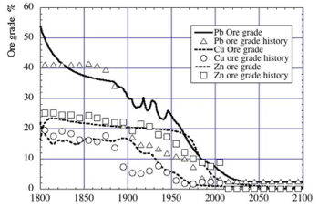
Figure 6.  WORLD model output mining rate for copper (a, left) and zinc (c, below left), total copper supplied to society and amount recycled (b, below right).  Decline in ore grades (d, bottom right); both WORLD model (lines) and observed ore grade (symbols) are in agreement.  Note: after 2050 recycling will be the dominant source of Zn and Cu. 

Iron, and steel made from it, constitute the most important metals for society.  Stainless steel is a composed metal mixture made from iron, manganese, chromium and nickel (50 million tons per year).  We also discuss aluminium (50 million tons per year), copper (16 million tons), and zinc (11 million).  Table 1 (online only) presents outcomes for peak production and time to scarcity, using our four estimation methods.  Analysis of the results in the table, shows that results obtained by using the different methods are in broad agreement.

An example of systems dynamics model outputs is given here in Figure 2 and Figure 3.  Figure 2 shows outputs from the WORLD model for iron, nickel and stainless steel.  When nickel runs out, high quality steels will be difficult to make.  Figure 3 shows the production rate for Mn-Cr-Ni stainless steel and Mn-Cr stainless steel without nickel.  It shows that when we run out of sufficient nickel, stainless steel will be substituted with a simpler quality, without nickel.  In the diagram, the recycling rate (30-60%) driven by price, was included.  It shows how the grades are predicted to fall in the next decades, driving up metal prices and making them more difficult to obtain. 

Figure 4 shows a simulation of primary aluminium production rate from 1900 to 2500, assuming the same extractable amount using the Hubbert’s (a) and the WORLD models (b,c).  The model was tested on how well it predicts the market price for aluminium.  Comparing aluminium’s ‘modelled’ price to real data, we get r² = 0.81 - a good validation of the dynamic model’s performance.  The model generates the price internally and uses it to feedback into supply and demand. 

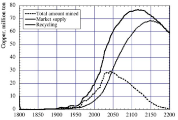
The interconnected flowchart for submodule BRONZE of the parent ores of copper and zinc, as modelled with the WORLD model, is shown in Figure 5, above.  The extraction of many technologically important metals are linked to the production of copper, zinc and lead and depend on their rate of mining.  Figure 6 shows the copper (a) and zinc (c) mining rate, the total amount of copper supplied to society compared to recycled metal (b).  Ore grades are predicted to fall (d), and our simulations closely match the actual ore-grade.  Historically, ore grade was compensated for by three factors: mechanisation (1900-1960), doing more of the work in low-wage countries (1960-2000) and automation (1990-2010).  As we run out of poor countries, where workers can be paid even less, and as energy costs increase, resource prices will rise. 

Figure 7.  Extraction rates for indium (a, left) and germanium (b, below right) from the WORLD model compared (lines) with actual extraction (open circles). 

Figure 7 shows further outputs from the WORLD model compared with actual extraction rates for indium (a) and germanium (b), two examples of metals vital to present and future technologies.  These metals are all dependent on mining of polymetallic ores containing copper, zinc and lead, and will reach peak production when copper, zinc and lead mines reach their peak. 

Figure 8 shows GOLD model (a WORLD submodel) assessment for gold production from mines (a); the dots represent observed data.  Gold has always been scarce, and its world use is therefore well adapted to scarcity and supply limitations.  The ore grade for gold over the last 100 years was modelled with good accuracy - showing that the models do describe what is actually going on (b).The WORLD systems dynamics models used here differ from traditional economic models in being strictly ‘causality based’ and ‘mass balance limited’.  Econometric models do not possess these properties, and so cannot predict prices.  Thus, they often fail and have limited predictive value. 

Figure 8. (a, left) GOLD model assessment for gold production compared with observed mining rate (dots).  (b, below right) GOLD model output for ore grade compared to historical ore grade (stars).   

Figure 9 shows that peak oil production was passed in the period 2008-2010.  Coal’s peak falls between 2015-2020, while peak energy will also occur then.  Peak wealth will arrive around 2017-2022, all based on 140 years of reservoir data and production rates³.  From that point on, we will no longer be able to take natural-resource-fuelled global GDP growth for granted.

Scarcity matters

Resource scarcity manifests itself in several ways.  The first will be price instability, which later becomes systematically higher prices.  Scarcity is also indicated by steadily sinking ore grades and increasing extraction costs, pushing price up.  This sometimes reduces demand, softening the blow.  Only at a much later stage does physical scarcity occur.  Platinum group metals are already scarce; price is already very high, and there are limits to how much can be supplied.  We may run out of money before we run out of materials.

Our resource Table (see below) shows four different estimations of risk for scarcity expressed as burn-off years, date for peak production and simulated peak supply to society - including conservation measures like recycling.  We have also assessed the overall risk at different time intervals considering all methods.  Estimates are consistent, and give scarcity risks very close to the present time.  Production of energy, metals for technology and infrastructure and phosphorus for food, are all closely linked and interdependent.  Many peak years occur within a few decades - making the appearance of problems much more risky and serious.  Just sitting and waiting may prove a disastrous strategy, leaving us no time for proper action until it is too late.  We cannot afford to fail on any of these resources, if the world system function is to be preserved.

A way forward?

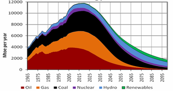Figure 9.  Fossil fuel production over time.  Note how dominant fossil fuels are and how small renewables are.  We will have to make do with very much less energy in the future.  (Association for the Study of Peak Oil, 2007).

The world is fast moving towards its limits.  We see peak behaviour in most strategically important metals, materials and fossil fuels that are fundamental to running our societies.  The continuing financial crisis since 2007 is not only a financial crisis, but one that showed how resource-backed economic growth cannot be sustained because of the physical limits of the world ^{5, 11}. 

In a world of limits, planning for further economic growth is a fool’s policy that will fail.  Many influential people remain stuck in denial of the finite nature of resources, and this is a significant problem.  A global population too large for a world where resource extraction has physical constraints will, most likely be one living in great poverty.  As resources decline and population rises, the situation will worsen.  It is one of the largest challenges ever faced by mankind. 

Long after all the gold mines have been exhausted, gold will remain with us because of recycling: we never lose any, always recycle it, and really look after it, because gold is scarce and has high value.  If this is possible for gold, then it is possible for other metals.  The key is systemic recycling for all metals and materials ^{17, 18}.

Every problem is a challenge, every challenge is an opportunity, every opportunity turned into a solution is a success.  Solutions must be found.  All of us, including geologists, need to rise to the occasion.  Business-as-usual is the worst case scenario.  There are many possible ways forward, many solutions to develop, and much change will be needed to make it all work.  For example, new development indicators are needed, that go beyond natural resource-fuelled GDP growth ^{17, 18}. 

Key policies needed include: Recycling, and developing models for an economy that converges within the sustainability limits.  It may be cyclic or steady state, but it must and will stay within the limits of sustainability.  If we do not do this, mass balance and thermodynamics will enforce it anyway.

We can all learn from Peter Seeger: ‘If it can’t be reduced, reused, repaired, rebuilt, refurbished, refinished, resold, recycled or composted, then it should be restricted, redesigned, or removed.’

References

1. Nørgård J.S., Peet J.  and Ragnarsdottir K.V.  (2010) The history of limits to growth.  Solutions, 1(2), 59-63, Feb-March.
2. Aleklett, K., Lardelli, M., Qvennerstedt, 2012.  Peeking at Peak Oil.  Springer.  Heidelberg.  335 pp. 
3. Campbell, C.  2013 Campbell's Atlas of Oil and Gas Depletion.  Springer Verlag, Berlin, 788pp
4. Meadows, D.L., Behrens III, W.W., Meadows, D.H., Naill, R.F., Randers, J., Zahn, E.K.O.  1974 Dynamics of Growth in a Finite World, 656pp.  Massachusetts: Wright-Allen Press, Inc. 
5. Meadows, D.  H., Meadows, D.  L.  Randers, J., Behrens, W.  1972 Limits to Growth.  Universe Books, New York.
6. Meadows D.H, Meadows D.L., Randers J.  1993 Beyond the Limits: Confronting Global Collapse, Envisioning a Sustainable Future.  Chelsea Green Publishing Company.
7. Meadows D.H, Randers, J., Meadows D.L.  2005 Limits to Growth, the 30 Year Update.  Earthscan, Sterling VA
8. Meadows D.H.  and Wright R.  (2008) Thinking in Systems: A Primer.  Chelsea Green.
9. Turner, G.M.  2009 A comparison of the limits to growth with thirty years of reality.  Socio-economics and the environment in discussion: CSIRO Working papers, Series 2008-2009
10. Turner, G.M., 2012 On the Cusp of Global Collapse? Updated Comparison of The Limits to Growth with Historical Data.  GAIA 2012; 21:116 –124
11. Sverdrup, H.  and Ragnarsdottir, K.V., 2014.  Natural Resources in a planetary perspective.  Geochemical Perspectives Vol.  3, number 2, 1-156.  European Geochemical Society.
12. Ragnarsdottir, K.V., Sverdrup, H, Koca, D.  2012 Assessing long-term sustainability of global supply of natural resources and materials.  Chapter 5; 83-116.  In; Sustainable Development–116.  Energy, Engineering and Technologies–Manufacturing and Environment.  Ghenai, C.  (Ed.).  www.intechweb.org
13. Sverdrup, H., Koca, D., Ragnarsdottir, K.V.  2013 Peak metals, minerals, energy, wealth, food and population; urgent policy considerations for a sustainable society.  Journal of Earth Science and Engineering.  2013b; 499-534.  ISSN 2159-581X
14. Heinberg, R.  2011, The End of Growth.  Adapting to Our New Economic Reality.  New Society Publishers, Gabriola Island, Canada.
15. Sverdrup, H., Ragnarsdottir, K.V., Koca, D., 2014.  On modelling the global copper mining rates, market supply, copper price and the end of copper reserves.  Resources, Conservation and Recycling  87:158-174, DOI: 10.1016/j.resconrec.2014.03.007
16. Sterman, J.  D., 2000.  Business Dynamics, System Thinking and Modelling for a Complex World.  Irwin McGraw-Hill: New York
17. Costanza R., Kubiszewski I., Giovannini E., Lovins H., McGlade J., Pickett K.W., Ragnarsdottir K.V., Roberts D., de Vogli R.  and Wilkinson R.  (2014) Development: Time to leave GPD behind.  Nature, 505, 282-285, January 16.   Hall, C.A.S., Balogh, S., Murphy, D.  J.  R.  2009 What is the Minimum EROI That a Sustainable Society Must Have? Energies, 2, 25-47.
18. Ragnarsdottir K.V., Costanza R., Giovannini E., Kubiszewski I., Lovins H., McGlade J., Pickitt K.E., Roberts D., de Vogli R., and Wilkinson R.  (2014) Beyond GDP.  Exploring the hidden links between geology, economics and well-being.  Geoscientist, 24(9), 12-17. 

The text supplied by the USGS (2004) as definitions is: Resource: A concentration of a naturally occurring mineral in a form and amount such that economic extraction of a commodity is currently or potentially feasible. Identified Resource: Resources whose location, grade, quality, and quantity are known or reliably estimated. Demonstrated Resource: Resources whose location and characteristics have been measured directly with some certainty (measured) or estimated with less certainty (indicated). Inferred Resource: Resources estimated from assumptions and evidence that minerals occur beyond where measured or indicated resources have been located. Reserve Base: That part of an identified resource that meets the economic, chemical, and physical criteria for current mining and production practices, including that which is estimated from geological knowledge (inferred reserve base). Reserves: That part of the reserve base that could be economically extracted at the time of determination. Marginal Reserves: That part of the reserve base that at the time of determination borders on being economically producible.  Undiscovered Resources: Resources whose existence is only postulated.

Authors

* University of Iceland, Reykjavik.  School of Engineering & Natural Sciences, Faculty of Earth Sciences, Askja, Iceland.