
Martin Geach * believes mwe must understand what happens inside the 'black box' if we are to ensure the quality of our outputs.
A defining characteristic of any geologist is the ability to think in three dimensions. From the creation of simple hand-drawn block diagrams to the production of comprehensive computer-generated ground models, we are often challenged to create a range of visual outputs that support our understanding of a 3D world. However, with the ever-increasing use of computer software packages to generate 3D ground models, do we need to take an important step back in order to appreciate the limitations and potential risks of the models we produce?
Visualisation
The importance of data visualisation has been rooted at the core of geology from its emergence as a practical science. Our evolution from William Smith’s seminal hand-drawn geological maps to the present-day integration of ground models in Building Information Modelling (BIM), demonstrates the diverse and challenging nature of the field in which we work. However, as professional ground practitioners, we must take steps to ensure the quality of our outputs. This is most important when applying computer-based algorithms to produce geological surfaces that are spatially incomplete and difficult to refine. In particular, I draw attention to the inherent limitations of geospatial interpolation techniques used in most software packages to create 3D surfaces.
In brief, geospatial interpolation is the technique used to join data points (such as strata depths from boreholes) in order to create continuous geological surfaces. Interpolation techniques range from: (i) Deterministic or Exact methods (e.g. Splines, Inverse Distance Weighting), where estimates of a variable at unknown locations are based on the spatial attributes of known locations, to (ii) Geostatistical / Inexact methods (e.g. Kriging), where variables at unknown locations are estimated, based on quantified values of autocorrelation between known points.
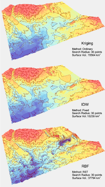
Plate 1 - Demonstrating the differences in interpolation techniques based on the approach adopted. Note the difference in surface volumes calculated from a fixed plane downward for each surface. IDW = Inverse distance weighting, RBF= Radial Basis Function. Interpolation conducted in a ARCGIS database applying standard toolsets.
Although you might not know it, geospatial interpolation is the backbone of any 3D model, yet the results generated from each technique can vary considerably. I demonstrate this fact simply in Plate 1 where a range of techniques are applied in a common software package. The dataset used is that of a river terrace record, where the distances between unknown points are typically less than 200m. You will note the range of surface volumes calculated from a known plane downwards, which represents the fundamental differences in the approach each technique adopts.
Errors
It is clear from this and many other examples that the complexity of interpolation can lead to notable errors when modelling geological data. This is most considerable when edge effects are poorly defined i.e., an interpolated surface is clipped to an arbitrary site boundary. However, when reading supporting documents to a 3D ground model, I wonder how often these inherent errors are appreciated?
Although I cannot doubt that 3D visualisation is a powerful tool taking geology into the 21st Century, we must not discard common sense (and our simple hand-drawn sections) and place too much emphasis on the creation of such models. As a minimum, geologists should be well aware of the limitations of all software and techniques and clearly identify the risk associated with such approaches.
* Dr Martin Geach works for Atkins as Engineering Geologist/Geomorphologist, Ground Engineering E: [email protected].