 Mike Stephenson* gives an insider’s view of the media frenzy surrounding the release of British shale gas figures
Just a few weeks ago there was a frenzy of activity leading up to the release of long-awaited resource estimates for shale gas in the north of England. The event placed geology right in the centre of the debate about what shale gas might mean for Britain. Suddenly geology really mattered to the ordinary man in the street. The question in many minds was: is there enough of this gas to make a difference to Britain? Or are we making a big fuss about nothing?
Previous gas company resource or ‘gas-in-place’ estimates had been on the large side, but other institutions (for example the American Energy Information Administration, EIA) put the figures lower. Some large oil and gas companies had basically written Britain off as a shale gas player. Environmentalists and industrialists alike complained: how could the figures vary so much? Confusion reigned. What we needed were reliable numbers.
MESSAGE
So the June 2013 BGS-DECC announcement was eagerly awaited. Until a week before the release only a few geologists in DECC and BGS had seen the figures. As overall manager of the project I was asked by DECC to give out the figures as part of a short presentation explaining the method. Behind the scenes I’d been exchanging endless different versions of a PowerPoint presentation with DECC to ensure that we could get the message just right.
The difficulty was with the size of the ‘resource’ figure, which is of course very large, more than 1300 trillion cubic feet (tcf). The main thrust of the presentation was thus, in management parlance, to ‘manage expectations’. We did not want headlines like ‘shale gas bonanza’ and ‘shale gas will pull Britain out of recession’. We wanted measured reporting with a careful explanation of the difference between ‘resource’ and ‘reserve’. Part of the process of releasing the figures had to include educating the media, together with a clear as possible presentation of the facts. So the presentation that we prepared contained lots of ways of explaining the difference between resource and reserve and lots of words of caution. (You can judge for yourself whether the message got out!)
METHOD
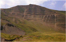
But back to geology – how was the estimate made? Anyone who has wandered the moors of the Pennines will know that there’s a lot of shale about. It’s one of the most common sedimentary rocks and up in Bowland or Kinderscout, if you are not standing on sandstone, you are probably on shale. But as any Carboniferous geologist will tell you the shales were deposited in a complex of rifting basins lying across central Britain during the Visean and Namurian. Some shales were deposited ‘syn-rift’, others ‘post-rift’.
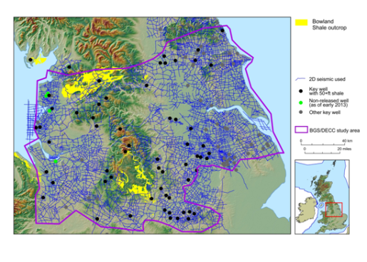 Picture: Area and key data for the BGS-DECC shale gas resource estimate
The key to making the estimate was to calculate a figure for the volume of shale in the chosen area (between Scarborough and Nottingham in the east, and between Lancaster and Wrexham in the west). To get this we built a 3D static model using 64 key wells and 15,000 miles of seismic, as well as years of data from shale outcrops. The surprise for all the geologists – and perhaps a primary reason for the size of the figure - is the thickness of the unit that we chose to define as prospective shale.
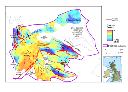 Picture: Thickness of the Bowland-Hodder unit
In the report (which you can download at www.gov.uk/government/publications/bowland-shale-gas-study) we called this the ‘Bowland-Hodder unit’. It is up to 5000m thick in basin depocentres (e.g. the Bowland, Blacon, Gainsborough, Widmerpool, Edale and Cleveland basins;) and contains quite high total organic carbon (TOC) levels (1-3%, though this can reach 8%). We know that these shales are capable of generating gas because there are conventional oil and gas fields in and around most of the basins and offshore.
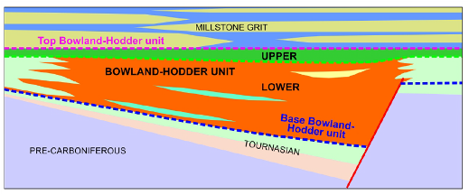 Picture: Schematic of the upper and lower parts of the Bowland-Hodder unit
The upper post-rift part of the Bowland-Hodder unit is laterally continuous, with organic-rich, condensed zones that can be mapped, even over platform highs. There is a lower, underlying, syn-rift unit, expanding to thousands of feet thick in fault-bounded basins, where the shale is interbedded with mass flow clastic sediments and re-deposited carbonates.
Once we had the volume in cubic metres of the two components of the Bowland-Hodder unit, we had to multiply by an estimate for the amount of gas that a typical cubic metre might contain. This and a ‘Monte Carlo’ simulation gave us an in-place gas resource for the upper Bowland-Hodder unit of 164 to 447 tcf and a range of 658 to 1834 tcf for the lower thicker unit. The map shows the prospective parts of the lower and upper Bowland-Hodder unit superimposed.
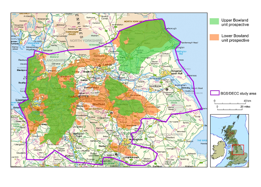 Picture: The prospective areas.
PRESENTATION
And so to the presentation of the numbers. On the morning of 27 of June a BGS team gathered in Whitehall at a press conference into which around 100 journalists were packed. The top table included me (as presenter of the figures), Ed Davey (Secretary of State for Energy and Climate Change) and Michael Fallon (Business and Energy Minister).
Davey opened the proceedings with a brief introduction to the Government’s Energy infrastructure plans. Fallon introduced shale gas, saying that today was “the day that Britain gets serious about shale gas”. Then I gave the presentation. Some of the numbers had already been leaked before the meeting, but I still think that journalists were surprised at their size. I spent most of the six or seven TV interviews that were held after (in the street outside the DECC building) explaining why these big figures had to be taken in context.
Apart from the excitement of the day, two things emerged: the importance of geology and the importance of independent institutions to provide trusted numbers. Whether you believe Michael Fallon or not about the prospects for shale gas in Britain, having figures that have been rigorously calculated and transparently presented helps to ‘steady the pulse’ of the nation and provide a base from which to make policy or investment decisions. The work underlines how relevant a geological survey is to a nation’s business.
BGS is probably the only institution in the country that could have provided this service - with its data holdings, breadth of expertise, and most of all its independence and even-handedness. No one – from the Secretary of State, to journalists, to industry, to the public, to NERC - can doubt the value of ‘public good’ geological research.
Having said all this, there are some things we can never get right. In the newspaper reports I read after the event, nearly all confused ‘resource’ and ‘reserve’! Some compared the UK’s shale gas with North Sea conventional gas reserves, and one reporter compared Lancashire shale with the Pars fields in Qatar and Iran, saying that northern England might be the next Middle East!
It just goes to show that you can lead reporters to data, but only editors and proprietors can tell them what to write!
* Prof. Mike H Stephenson is Director of Science and Technology, NERC British Geological Survey
Acknowledgements
The DECC report is: Andrews, I J 2013 The Carboniferous Bowland Shale gas study: geology and resource estimation. British Geological Survey for Department of Energy and Climate Change, London, UK.
The BGS team included: Ian Andrews, Sue Stoker, Mike Sankey, Chris Vane, Kevin Smith, Mike McCormac, Vicky Moss-Hayes, Nigel Smith, Ceri Vincent and Nick Riley. Toni Harvey led the DECC team.